multi-phase linear regression
Example output from stats_regress2lines.m
corresponding with this example plot shown on the article webpage:
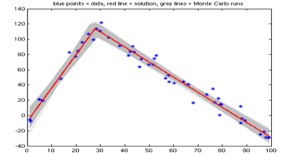
Statistics for two-phase straight-line regression:
Model is two lines:  y=a1*x+b1 and y=a2*x+b2, intersecting at x0.
Playing with synthetic data; true model for m=[a1,b1,a2,b2,x0] is:
        5        -10         -2      168.5      25.5
Note we assume that the data noise are Gaussian with constant unknown stdev.
Known population standard deviation for synthetic true data = 10
Data sample standard deviation s computed from residuals = 7.67
Solution via two-line iterative regression for m=[a1,b1,a2,b2,x0]:
    4.397     -7.551     -1.981      169.2     27.72
Associated stdevs for m=[a1 b1 a2 b2], computed from covariance matrix below:
   0.2438      4.048    0.05767      3.915
Model covariance matrix for m=[a1 b1 a2 b2], computed from s and optimal G :
  0.05942    -0.8261          0          0
  -0.8261      16.39          0          0
        0          0   0.003326    -0.2141
       -0         -0    -0.2141      15.33

SStotal should equal SSmodel+SSresids, so SStotal-SSmodel-SSresids should = 0:
SStotal = 92502.012
SSmodel = 89797.4483
SSresids = 2704.5637
SStotal-SSmodel-SSresids = 6.5438e-10  <-- (consider: close enough to zero?)
Coefficient of determination R^2 = SSmodel/SStotal = 0.97076

Starting 10000 Monte Carlo runs to compute Cm (each run calls regress2lines)
10%... 20%... 30%... 40%... 50%... 60%... 70%... 80%... 90%... 100%...

Full-scale Monte Carlo means for m=[a1,b1,a2,b2,x0] via 10000 fwd problem runs:
    4.392     -7.524     -1.984      169.4     27.77
Associated standard deviations for m=[a1 b1 a2 b2 x0] based on cov matrix above:
    0.259       4.11    0.05853      3.993    0.8273
Monte Carlo model cov matrix for m=[a1 b1 a2 b2 x0] via 10000 fwd problem runs:
  0.06706    -0.8849   0.001022   -0.08132   -0.1616
  -0.8849      16.89  -0.009249     0.7083     1.279
 0.001022  -0.009249   0.003426    -0.2218  -0.02291
 -0.08132     0.7083    -0.2218      15.95     1.782
  -0.1616      1.279   -0.02291      1.782    0.6844