This Matlab/Octave package calculates Tikhonov-regularized, Gauss-Newton nonlinear iterated inversion to solve the damped nonlinear least squares problem. Among other applications, these are problems commonly discussed in geophysical inverse theory settings.
While Matlab's optimization toolkit contains
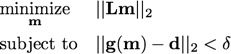
lsqnonlin, it does not inherently include the Tikhonov regularization and is only the optimization part, whereas inversion also requires uncertainty quantification. InvGN is for weakly nonlinear, Tikhonov-regularized, inverse problems (so includes solution uncertainties and resolution quantification) and parameter estimation problems, handles both frequentist and Bayesian frameworks, and also works in Octave.The damped nonlinear least squares problem is:
For appropriate choices of regularization parameter lambda, this problem is equivalent to:
where delta is some statistically-determined noise threshold, and also to:
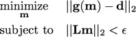
where epsilon is some model norm threshold.
The damping level (regularization parameter lambda) is solved for by the L-curve method (see e.g. Hansen 1987), and the L-curve is one of InvGN's outputs.
The code is based on material from:
- Professor Ken Creager's ESS-523 inverse theory class, Univ of Washington, 2005
- RC Aster, B Borchers, & CH Thurber, "Parameter Estimation and Inverse Problems," Elsevier Academic Press, 2004.
- A Tarantola, "Inverse Problem Theory and Methods for Model Parameter Estimation", Society for Industrial and Applied Mathematics, 2005.
- PC Hansen, "Rank-Deficient and Discrete Ill-Posed Problems: Numerical Aspects of Linear Inversion," Society for Industrial Mathematics, 1987.
- PE Gill, W Murray, & MH Wright, "Practical Optimization," Academic Press, 1981.
InvGN is compatible with Octave (version >3), but to handle a few minor remaining differences between Matlab and Octave, do note the "usingOctave" flag among the options listed at top of the InvGN.m script. Perhaps in future versions INVGN will allow these options to be set via keyword/value pairs in the input argument list, but not implemented yet.
The function call is designed to allow use on both (weakly) nonlinear and linear problems, both regularized (inverse) and non-regularized (parameter estimation) problems, and both frequentist and Bayesian problems, and using a user-supplied function for the Jacobian matrix of derivatives or internally calculating finite differences, as determined by the form of its input parameters.
USAGE:
[ m, normdm, normmisfit, normrough, lambda, dpred, G, C, R, Ddiag, i_conv ] = ...
invGN( fwdfunc, derivfunc, epsr, dmeas, covd, lb, ub, m0, L, lambda, maxiters, useMpref, verbose, fid, vargin );
Just as a few examples to demonstrate this idea of different inputs causing different mode of computation: If
derivfunc is not a string or @functionhandle to a user-specified function but rather =[], then invGN will internally calculate finite differences. Setting matrix L or scalar lambda to zero cancels the regularization and simple (overdetermined) parameter estimation is computed. And the useMpref flag allows to choose between the cases of frequentist estimation with or without a "preferred model" (minimizing distance to), or Bayesian estimation; in the Bayesian estimation case the outputted model covariance matrix is the Bayesian posterior rather than the frequentist covariance with resolution matrix. In any case, all these options are thoroughly described in the manpage included in the package, along with definitions and discussions of all the input and output parameters. This webpage is purely an introduction and won't describe most of the parameters as that manpage does. Here are a few of the examples from that manpage:A FEW EXAMPLE CALLS:
(Leaving off the output part "[ m, normdm, normmisfit, etc. ] =" which is the same for all cases. The parameter defn's in the manpage will greatly help to understand these examples.)
Regularized frequentist inversion with auto-chosen lambdas (numlambdas of them for an L-curve) and using finite differences for the Jacobian matrix:
invGN( fwdp, [], epsr, datameas, -invcovd, lb, ub, minit, L, -numlambdas, 0, maxiters, 3, 1 );Nonlinear parameter estimation with finite differences for the Jacobian but no regularization:
invGN( fwdp, [], epsr, datameas, -invcovd, lb, ub, minit, zeros(size(L)), maxiters, 3, 1 );Frequentist nonlinear problem with preferred model:
invGN( fwdp, [], epsr, datameas, covd, lb, ub, mpref, eye(M), -numlambdas, 1, maxiters, 0, 1 );Bayesian nonlinear problem:
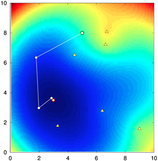
invGN( fwdp, [], epsr, datameas, covd, lb, ub, mprior, chol(inv(Cprior)), maxiters, 0, 1 );USE EXAMPLE #1: NONLINEAR PARAMETER ESTIMATION
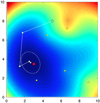
This demonstration is a 2-model-parameter parameter-estimation problem, the Lab 4 problem written for the Geophysical Inverse Theory class at University of Washington. It's a source-location problem for which the assignment was to calculate and plot the objective surface, and then calculate and plot the Gauss-Newton estimation steps leading to the solution point (the minimum of the objective surface).
(sorry, still finishing filling in the content below... will be done soon!)
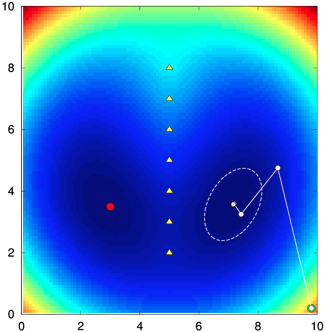
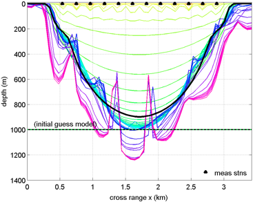
USE EXAMPLE #2: INVERSE PROBLEM (WITH REGULARIZATION)