
Beamforming is a general signal processing technique used to control the directionality of the reception or transmission of a signal on a transducer array.
Using beamforming you can direct the majority of signal energy you transmit from a group of transducers (like audio speakers or radio antennae) in a chosen angular direction. Or you can calibrate your group of transducers when receiving signals such that you predominantly receive from a chosen angular direction. The physics and math are essentially the same for both the transmitting and receiving cases, so I will concentrate on the transmission case to explain the concept further. I should mention as well that there are a few general approaches to directing this signal energy, but by far the most common is having a slightly different signal go out of (or into) each transducer in your group; this is the approach I discuss here. Another interesting but less common approach is sending the same signal to all transducers but with varying information encoded by frequency in that signal, requiring a broadband signal - this is called using a "blazed array". However, I don't discuss that approach here.
The basic point in beamforming is, when you set multiple transducers next to each other sending out signals, you're going to get some kind of interference pattern, just like you see in a pond when you throw several stones in at once and create interfering ripples. If you select the spacing between your transducers and the delay in the transducers' signals just right, you can create an interference pattern that's to your benefit, in particular one in which the majority of the signal energy all goes out in one angular direction. To show this is true and what this looks like, I'm going to show a really simple example, using some sin waves being emitted from several point sources as seen below. In my example, to keep things simple I use a straight line array of transducers within a 2D field, although that introduces some direction ambiguity issues (as you'll see that in a moment). This direction ambiguity is remedied by not putting the transducers all in a line (for 2D), but first things first.
The sin waves below are moving out from all the sources just like ripples do in a pond, and I'm going to assign variables to my arrangement rather than numbers, so that I can change them and see how those changes affect my overall resulting interference pattern. So note I have a constant spacing d between each of my transducers (point sources here), and an origin of some coordinate system centered on the center transducer. I'm going to use a polar coordinate system because I'm interested in seeing how my interference pattern affects things angularly, so note at each point theta, r in that coordinate system I have a particular wave amplitude. Theta is measured counter-clockwise starting from zero at the axis arrow on the right, matching the usual convention.
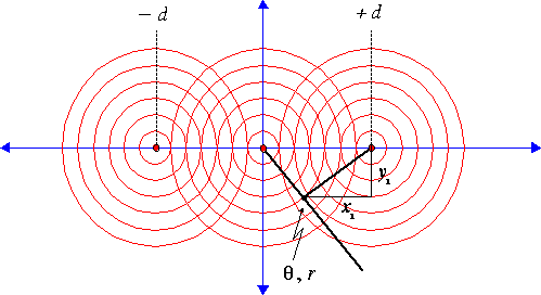
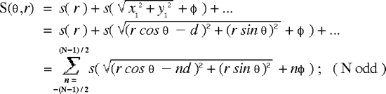
What I want to do given this arrangement is to find out what the interference pattern looks like when I zoom out from this picture, so I want come up with a mathematical expression for total amplitude at any radius and angle away from the origin. This total amplitude is going to be some kind of sum of the signals from the transducers, and I want this expression to include variables d for distance between transducers and phi for time delay given to each transducer's signal so I can vary these later and see the effects. My convention for this delay will be that the center transducer has no delay, the transducers to the right will have integer multiples of delay phi, and the ones to the left will have negative integer multiples of delay phi. So if phi is zero, there is no delay and the signals from all the transducers come out in phase.
In the expressions below, S(theta,r) is the signal strength (the color on the plots) as a function of azimuth and radius. It depends upon the signal function itself, s(t). (Many apologies for the S and s confusion that came up with some readers, but the two are different functions.) Notice that for the example, the value used for t is simply distance from the source of the respective signal. So if we have, say, three sources interfering to create a beam pattern, we then have three s(t) functions which are summed.
In the plotted examples I've made, I've simply used a sin() function for s(t), but it could be anything. Arrays of radio towers for example may send out their radio signal as s(t), spaced in location and time, to narrow a beam toward a city rather than waste power on radio signals radiating in other directions away from the city.
Okay, so now given that overview let's look at some plots from a set of Matlab scripts I wrote that implements these equations.
The Matlab scripts that created these plots are called polar_interference.m, polar_ang_avg.m, S.m, and sig.m (found in my GitHub account at https://github.com/aganse/tutorial_beamform). The S.m file here is the S(theta,r) function from the math expression, and the sig.m file is the s(t) function. These scripts loop over a number of the examples below, and write .png graphics files of the plots to the current directory. (.png files are similar to .gif files and are viewable in most graphics apps including your web browser.)
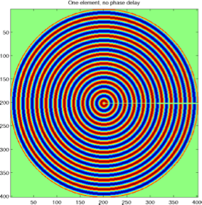
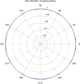
In the first case we have just one source in the middle, and as we expect we have just concentric ripples emanating from it. In the wave field plot on the left we have red showing positive values of the field and blue showing negative values; green is zero. In the polar "beam pattern" or "polar response" plot on the right, we have a normalized angular average of the wave field, so that there's one average value for each direction and the maximum one over all the directions is set to equal one. It doesn't show much here because the signal in this example is the same in all directions. But this type of plot is common when showing beamforming results, and as you will see farther below it more clearly shows the "sidelobes" that are the result of an imperfect (but still plenty useful) directionalizing process.
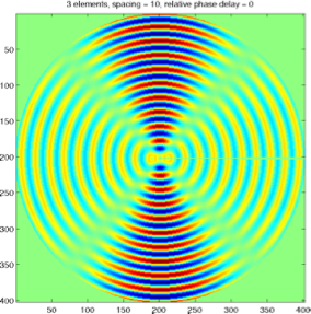
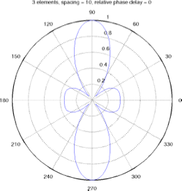
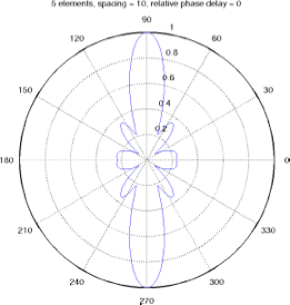
Now we have three sources, set 10 units apart on the x axis - one source in the middle and one on each side. (Sorry I didn't include the sources themselves on the plots, but you can sortof see where they would be, given the axes labeling and the little circular features in the ripples at the plot center.) The three sources are all pinging at the same time, however - no "phase delay" between them - and so the beam direction is orthogonal to this linear array of sources. Note how the angular average plot on the right now shows directional dependence with two big and two small lobes. The big lobes in the polar average plot are called "beams", ie the main directions we are interested in. As seen farther below, we can "steer" these beams in a desired direction to preferentially send or receive a wave in that direction. Note that the directionalizing process isn't perfect; the interference pattern has additional ups and downs which you can see in both plots, and which appear as "sidelobes" (the lesser lobes to the left and right) in the plot. Finally, note too the ambiguity in direction here - the array is in a line, so we get a beam both up as well as down. That means when we receive a signal we won't know if it came from up or down, and if we transmit a signal we will be transmitting in both the up and down directions.
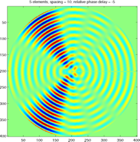
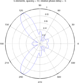
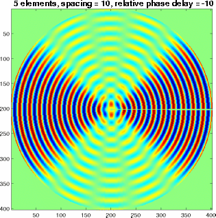
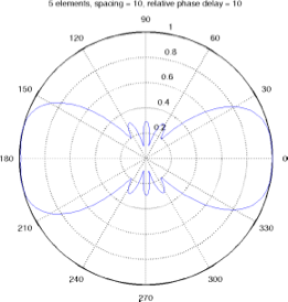
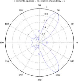
Now we have five sources, set 10 units apart on the x axis - one source in the middle and two on each side. This time the sources don't all ping at the same time. They have a five-unit time delay (say 5ms) between them such that the center source pings on time, the first source to its right pings 5ms early, the second source to the right pings 10ms early, the first source to the left pings 5ms late, and the second source to the left pings 10ms late. This results in a warping of the interference pattern, in a way that creates a beam that is "steered" in a particular direction. We can see this in the polar response plot on the right as well, although we see that the sidelobes in this case, while small, have a more complicated structure than before. Note again the directional ambiguity, so that while I tried to steer my source to a 120 degree beam, I also get a beam at 240 degrees. For a linear (or for that matter planar) source there's no direct way that I know of to get around this. But on a practical side there are engineering ways of addressing the issue; for example you could make a baffle that sits on one side of the array and knocks the transmission way down on that side of the beam pattern.
Just for fun I put a bunch of these together in an animation to show a beam being steered around...
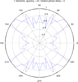
And lastly, here are some additional beam patterns calculated from my Matlab script. Note you can have different "beam widths" as well as directions, and the sidelobes can sometimes become so large as to make a complete and useless mess out of things.
Again, the Matlab scripts that created these plots are called polar_interference.m, polar_ang_avg.m, S.m, and sig.m (found in my GitHub account at https://github.com/aganse/tutorial_beamform). These scripts loop to create many of the examples above, and write .png graphics files of the plots to the current directory. (.png files are similar to .gif files and are viewable in most graphics apps including your web browser.)
However, the animated plot was pieced together manually from a set of these still plots using a separate graphics program. You're on your own for that.