A classic textbook on predictive filters is Applied Optimal Estimation, editted by Gelb (1974). In section 6.1 of that book are two simple radar tracking examples (6.1-2 and 6.1-3) which demonstrate several nonlinear filters. I've programmed up those examples into a Matlab script called gravdragdemo.m and added a few other filters to compare and contrast them in both linear and nonlinear cases. Here are recreations of the figures in Gelb for examples 6.1-3 (2D nonlinear measurements case) and example 6.1-2 (1D linear measurements case) respectively:
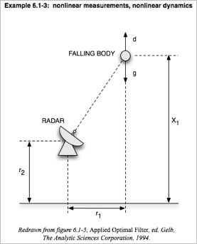
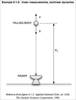
These examples use radar ranging to estimate the elevation, downward velocity, and drag coefficient for a falling body as functions of time. These three values are collected into a 3x1 vector called the state vector x, again a function of time. The two examples are related: example 6.1-3 has a 2D arrangement to create nonlinear measurements with respect to x. Example 6.1-2 is a special case of 6.1-3 in which the problem has collapsed to 1D by letting r1 and r2 shrink to zero, causing the measurement relation to become linear with respect to x. The dynamics of both examples in the book are nonlinear because they include air drag (x3), which depends on velocity (x2). The equations for this problem are pretty basic:
definition of state parameters:
dynamics equation:
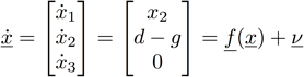 (where the v is the dynamical error or “plant noise”)
definition of drag d and atmospheric density relating to it:
measurement equation:
Note I actually don't redo the book's example 6.1-3 exactly; I still use x3=β for both examples, and use the initial conditions from example 6.1-2 for both problems. This linked the two examples better, letting me simply zero out r1 and r2 to collapse 6.1-3 down into 6.1-2.
In the Matlab script we can choose whether to make the measurements a linear or nonlinear function of the states by setting r1 and r2 to be nonzero or zero. We can also specify whether to make the dynamics linear or nonlinear by setting the forces on the falling body (drag d and gravitational acceleration g) to nonzero or zero. Granted, for the linear case it's a little strange because the "falling" body no longer even has gravity acting on it, but the idea was to have an example which kept at its initial velocity to make it linear - so sue me!
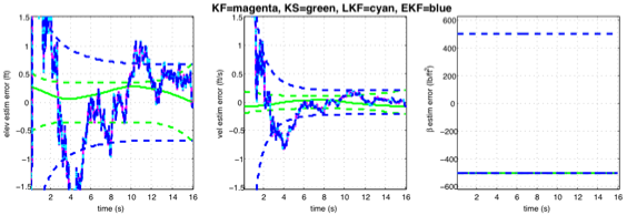
The point of running this script with its different settings is to compare the resulting plots showing how well the filter fared. A commonly seen plot in the filter community is the estimation error plot, which for a synthetic example shows error deviations from the known true state vector x as a function of time. The filters have a random element to them so the iterative paths toward a solution can jump around, but ideally those paths converge on the zero error line, meaning the filter converges to the true value. The fluctuating center line is the expected value (mean) state calculated by the filter minus the true state (only known in the synthetic problem), and the lines above and below forming a corral are the plus- and minus-one standard deviation lines. Here's an example of what the plots look like, and we'll come back to discuss the details of this particular plot a little farther below.
An example of the estimation error plots the script uses to compare the filters for a synthetic problem:
We see at the top of the script which of the filters (or smoother) are in used in a given run:
% - Kalman Filter (KF),
% - Kalman Smoother (KS),
% - Linearized Kalman Filter (LKF),
% - Extended Kalman Filter (EKF),
% - 2nd order EKF (EKF2)
The initial conditions for both examples 6.1-2 and 6.1-3 here were taken from examples 6.1-2 in the book, and the initial covariance matrices had to be estimated based on the book's figures 6.1-3 and 6.1-4. I also added a Q matrix option (the book's examples assumed Q=0 and so well leave the Q "turned off" for now) and estimated the time increment T from the book's plots, as it wasn't given:
% Initial conds and setup is the same for both 1D & 2D problems.
% (these default values here are taken from book):
x0true=[1e5+100,-6000+350,2500+500]';  % = elevation(ft), velocity(ft/sec), drag coeff
x0guess=[1e5,-6000,2500]';  % note this will cause LKF's xbar to cross zero a little early...
P0=diag([500,2e4,2.5e5]);
Qon=0;  % multiply this scalar times the Q matrix to "turn it on&off" (ie 1=on,0=off)
        % Gelb examples both have Q=0; you can change Q down in getQ() function, default is 1e2*I)
R=1e2;  % note meas noise cov matrix is a single scalar variance in this problem

% Note all filters in this script assume equally-spaced time points:
T=.01;  % Timestep for discretization of continuous functions of time.
        % Note the Gelb book examples very likely used a timestep of order
        % 0.01 and then only plotted every 10th point or so.
timerange=0:T:16;  % or try 17.7;  % both in sec
It was mentioned above that the script can handle both linear and nonlinear dynamics and measurements for comparison of filters. Let's initially set the problem to its simplest state - completely linear in both measurements and dynamics - using these lines found near the top of the script:
nonlineardyn=0;  % problem dynamics: 1=nonlinear (both Gelb examples), 0=linear (to try KF)
nonlinearmeas=0;  % problem measurements: 1=nonlinear (Gelb ex6.1-3), 0=linear (Gelb ex6.1-2)
We can specify which filters to turn on together in the script as follows. Let's turn on the Kalman Filter, Kalman Smoother, Linearized Kalman Filter, and Extended Kalman Filter:
% Choose which filters to try:  1="on" and 0="off" on all these...
runKF=1;
runKS=1;
runLKF=1;
runEKF=1;
runEKF2=0;
We see in the resulting plot that for the linear problem, the Kalman Filter (KF) converges to the true parameter values (within the standard deviations shown in the dotted lines), and that the Linearized Kalman Filter (LKF) and Extended Kalman Filter (EKF) exactly match it in this problem because they both use linearization techniques which will equal a linear filter if the problem is linear. Note that the last point of the Kalman Smoother (KS) result equals the last point of the filters in a linear problem, and that the smoother has considerably less uncertainty than the filters because it returns to readdress all the data points again. The plot of the third parameter β shows nothing in this problem because drag is wired to zero in the linear problem, so β remains at its initial guess value.
Linear measurements and linear (trivial!) dynamics:
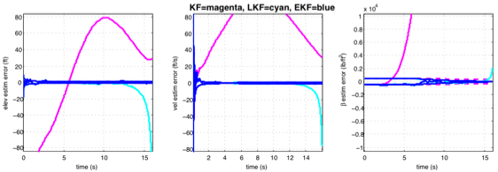
Next we keep the measurement function linear but now include the drag, making for nonlinear dynamics. Since the drag is now included the third parameter plot is now active. We compare the LKF and EKF, two nonlinear filters, and see that the EKF performs better. The LKF does not handle the nonlinearity as well and eventually diverges more in its error because all its linearization points are precomputed before the filter run, whereas the EKF linearizes on the fly.
Linear measurements and nonlinear dynamics:

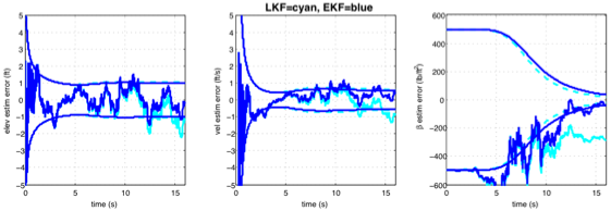
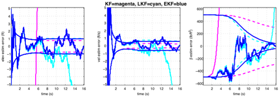
Now let's bring in the rest of the nonlinearity - the measurements are nonlinear too now via the 2D geometry. By the way, we didn't try the plain linear Kalman Filter on the nonlinear problem on the last plot, so let's try that here. We see here that it blows it big-time (it's the magenta line), as seen in the zoomed-out plot next. The LKF diverges after a while too, but at least it's far better than the KF. The EKF tracks the process better and converges to fluctuations within the uncertainty.
A note about those uncertainties though. For the linear problem the standard deviations (and unplotted covariances) are exact, in the sense that given Gaussian noise on the measurements and a linear problem, the uncertainties on the estimated states will be Gaussian. But a nonlinear problem will instead map those Gaussian distributions into non-Gaussian ones. So at each time step when the LKF or EKF (or 2nd order EKF farther below) bases its next step on just the mean and covariance, it's leaving out information and is heading off in somewhat the wrong direction, as well as misrepresenting the uncertainties at a given time. So instead of relying on the EKF's standard deviation lines in these plots, the Gelb book recommends running say 100 or 1000 Monte Carlo simulations and estimating the standard deviations that way. There are plots of Monte Carlo based uncertainties for these examples in the Gelb book, but I did not implement the Monte Carlo part in my Matlab script.
Nonlinear measurements and nonlinear dynamics:
Same problem but zoomed in:
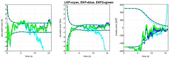
Finally, below we see the results of the 2nd order EKF in comparison to the EKF results. The problem is the same one as above but the plots show a different run which means a new instantiation of the filters' random walks. While the plot here looks like it shows that the 2nd order EKF converges faster than the EKF, really the way to show this would be to compute the Monte Carlo based standard deviations discussed above, as the Gelb book does. Maybe I'll add this into my Matlab script in the future. Meanwhile, perhaps you'll find the script fun and instructive to play with as is.
Nonlinear measurements and nonlinear dynamics again, just a different instantiation to show 2nd order EKF now:
Again, you can download my gravdragdemo.m script here, and it merely implements the two simple radar tracking examples (6.1-2 and 6.1-3) in Gelb. Have fun!