
New analyses of radio-science gravimetry of icy outer-solar-system moons
 The nature of an icy satellite's interior relates fundamentally to its composition, thermal structure, formation and evolution history, and prospects for supporting life. Gravity measurements via radio Doppler information during spacecraft flybys are an important tool used to infer gross interior structure of these moons. Liquid water and ice layers have previously been inferred for the interiors of Jupiter's icy satellites Europa, Ganymede, and Callisto on the basis of magnetic field measurements by the Galileo probe, and on Europa and Callisto induced magnetic field signatures measured by the Galileo probe provided strong evidence for an ionic aqueous ocean.
 Oceans in icy satellites present the possibility of habitable environments removed from the conventional “habitable zone.”' Given the possibility of liquid water in multiple icy satellites and outer solar system objects, icy satellite oceans could be more common than oceans on terrestrial planets. Very deep oceans are likely complex chemically and dynamically. The presence of a fluid layer determines the nature of heat transport from the satellite's interior, with the interplay between pressure, temperature, and composition potentially limiting rapid advective cooling.
 Signatures of hydrothermal activity and ocean/ice-shell interactions may cause thermal, compositional or density anomalies that can be detected remotely. Identifying internal structure in ocean-bearing icy worlds has implications for understanding their thermal and compositional evolution.
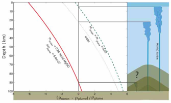
 For example, a seamount feature within in Europa, as pictured, would affect the circulation of fluid in a liquid ocean by impinging on stratified layers, and possibly by acting as a focus for hydrothermal activity. This plumes figure illustrates how plume buoyancy is affected by ocean and plume composition, and by depth-dependent thermodynamic properties (e.g. density) of those solutions.
We have lately been examining publicly available Europa Clipper (next proposed Europa spacecraft) mission study technical data to address the ability of gravimetry to resolve structures in Europa’s interior, such as large-scale diapirs, brine and melt pockets and large (>10 km) seamounts. We use geophysical inverse theory tools in the experiment-design / mission-planning stage to calculate the location-dependent resolution of features in the H20 layer inferred by gravimetry. We also use forward-modeling analysis to estimate feature-size detection thresholds. Instead of estimating a few spherical harmonics of gravity potential, we use the extensive flyby coverage to try to explore what scales of possible density anomalies in an H20 layer may be resolved against the background of those spherical harmonics of gravity potential. Forward as well as the inverse analysis aims to bound the true sizes and locations of density anomalies that might be discovered in an actual Europa Clipper mission.
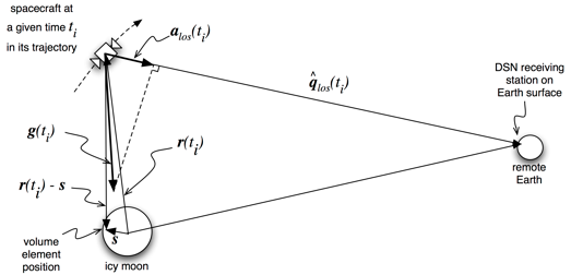
As a spacecraft flies past an icy moon or any other planetary body, density anomalies in the body tug on it and cause “wiggles” in its trajectory. These wiggles have a component in the line-of-sight-to-Earth direction, and so cause minor Doppler shifts in the radio frequency signal being sent to Earth. Measurements of these Doppler shifts over time can be inverted to infer the density anomaly distribution.
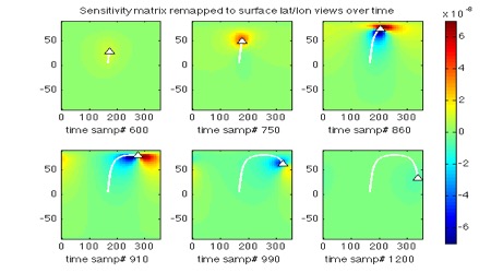 Part of the process involves solving for sensitivities of the measured radio Doppler signal to the icy moon crust’s density anomaly structure over time in the trajectory. A map plot example of these sensitivities follows intuition. There is a negative and a positive tug by a possible anomaly in any given position as the spacecraft flies past, and these tugs (and thus sensitivities) are stronger with lower altitude as the spacecraft trajectory is near its closest approach in the flyby (the apex of the U shape in the surface projection of its path).
In doing these calculations, the moon is actually parameterized in a geodesic grid so that wrap-around at the poles and grid weighting with latitude are not issues. This geodesic grid is the reason the rectangularly mapped results below have somewhat "ragged" edges at the sides.
 |  |  |
As one might assume, there’s only so much information about such anomalies (or structure of the body in general) that can be obtained from the measurements. This limited information presents itself in the form of limited resolution of features detected. Natural questions here are: what’s a physically and statistically rigorous way to assess this limited resolution, and can it be done before the actual measurement in order to help plan the best trajectory geometry to obtain the best resolution possible given tradeoffs with other mission needs? The answer to that second question is “yes”.
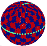
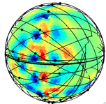
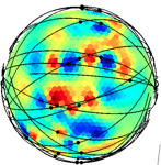
On the intuitive side, one can calculate a synthetic inversion, in which one makes up a density anomaly structure for the moon, uses it to create synthetic data which gets noise added to it, and then this noisy synthetic data is inverted to see how much of the structure is resolved by the inversion. A common test of this sort is called the “checkerboard test” where the density anomaly structure is a checkerboard pattern. (It’s a test pattern -- we don’t assume this is really what the moon structure is like!) As we might expect, in the inversion result we can see that near the apex of the flyby path the structure is inverted pretty well, farther out on the flyby path the structure is inverted somewhat well, and away from the path virtually nothing is recovered of the checkerboard. In other words, the resolution of the inversion is location-dependent. The globe figures above are low-res 3D representations of such tests, and below are higher-res versions depicted in a Mercator projection:
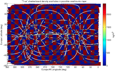
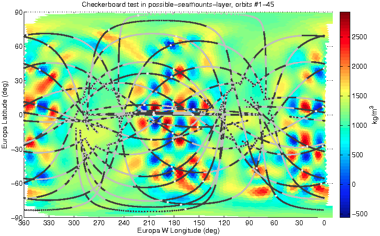
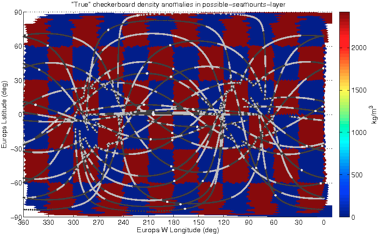
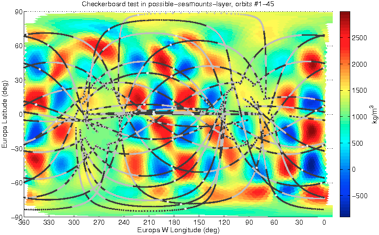
In these checkerboard tests above, the red-and-blue rectangles are two sizes of grids, and the more colorful plots show how the inversion is able to resolve those grids again from synthetic data produced from those grids. The gray-and-black curves are the lat/lon projections of the flyby trajectories (gray/black = 500m intervals in altitude, white dots are lat/lon of closest approach). Note that some regions have poor resolution and others have better resolution, according to where the flybys were closest and overlapped; i.e. the resolution of the inversion is location-dependent.
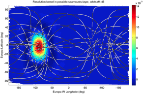
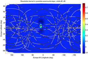
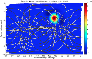
While the checkerboard tests are useful demonstrations, the resulting resolution matrix actually quantifies the resolution limits exactly for linear inverse problems such as this one, and it can be computed without the measured data (or synthetic checkerboard data for that matter). It contains lat/lon-dependent impulse responses of the inversion (“resolution kernels”, see figure at left), which show the averaging regions in which the inversion necessarily blurs the true real-world density anomalies due to ill-posedness of the inverse problem.
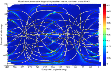
Since there is one of these resolution kernel maps for every single map location, a useful summarization quantity is the lat/lon map of the resolution matrix's diagonal (shown without and then with the lat/lon projections of flyby trajectories), with greater value at regions of good resolution:
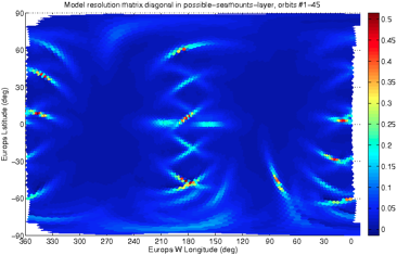
For a more intuitive and functional result, we are presently calculating cross-widths of each resolution kernel and plotting those as a function of map location, to compare more directly with our forward problem resolution results and other instrument coverage results, but that map will look very similar to the resolution diagonals map above. Not surprisingly, those resolution summary results bear some resemblance to patterns seen in coverage of other instruments - optimizing flyby geometry is crucial because so many instruments are sensitive to that geometry.
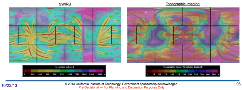
from public ICEE Team Welcome Briefing Notes from Europa Clipper Pre-Project Team, 2013, https://solarsystem.nasa.gov/europa/iceedocs.cfm, page 96
In summary: overall in this work we actually focus on two complementary types of analysis. The forward problem analysis addresses feature-detection thresholds, while the inverse problem analysis described above addresses what the measurements will be able to uniquely resolve. These analyses work together to bound the true sizes and locations of anomalies which could be detected in the actual mission, and where they could be imaged. This work highlights and quantifies the stringent limitations imposed by the ill-posedness of the problem upon the ability to uniquely localize and characterize the ice-layer anomalies we are so interested in.