
(In the time since I wrote this many years ago I discovered a more general framework that can also do this sort of problem - multivariate adaptive regression splines (MARS), for which there's a Python toolkit and a Matlab toolkit among others listed on the Wikipedia page (that link).)
An introduction to the problem
Standard linear regression fits a set of data points with a linearly parametrized polynomial (like
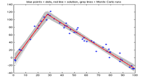
Figure 1. An example of fitting two straight lines to one's data using multi-phase regression. The gray lines in the background are 104 Monte Carlo fits based on different instantiations of the noise on the data points, used in estimating the statistics of the fit for this nonlinear problem. To get a feel for what the Matlab script stats_regress2lines.m (linked at right) calculates, check out the example output file corresponding to this plotted example.
The calculational concept behind finding a best multi-phase regression fit is related to that behind the basic linear regression fit taught in statistics 101, except now the problem has become nonlinear due to the unknown intersection point of the fit lines. This nonlinearity means the problem takes a little more work to solve, but that's what makes it interesting. The problem is continuous but nondifferentiable at a number of places due to the line intersections, and this messes up the local linearization approach often used for weakly nonlinear problems. The nonlinearity also complicates the interpretation of the statistics of the estimated parameters. (Just as with standard linear regression, the solution is an estimate and has an uncertainty associated with it.) However, these issues are not insurmountable.
Important Usage Note
This technique (and associated software below) fits two straight lines to your data points. But you should have some theoretical justification in your particular problem for your choice of fitting two straight lines instead of, say, a single exponential or polynomial. As a positive example of usage, a biologist who wrote me was modeling the change in body part size ratios of a certain insect. The insect had one constant growth rate (linear growth) in its larval stage and then a second constant growth rate in its adulthood, so the fitting of two straight lines to the size data points was a natural, justifiable choice. However, if your problem does not have two clearly identifiable linear regimes to it (or N curve regimes) then you likely should not use this method - perhaps Matlab's polynomial-fitting routine
polyfit may be useful, or maybe your system is exponential. Whatever it is, I recommend that the model you choose has some physical or natural basis in your problem.Matlab Code
You are welcome to try my Matlab script
regress2lines.m which implements a two-phase version of this regression - fitting two straight lines with an unknown intersection point to a set of noisy data points. Statistics of the solution estimate to this nonlinear problem are explored in stats_regress2lines.m, which calls regress2lines.m many times in Monte Carlo simulation (watch out, note that can potentially take a while to run). It also plots the result as seen in the example in figure one at left. These scripts and the example output are available in the MultiRegressLines.matlab repository in my GitHub account.However, this routine has a some important caveats. These caveats mean that for particular situations the fit result will be completely wacky. If you do not want to implement the additional formulations discussed in the references to handle this, you must be sure to plot and visually check that your fit result looks sensible every time you run it. I.e., this code is not good for automated results.-->
Calculational procedure
The problem definition is to solve the following:
• Given xdata(1:n),ydata(1:n)
• Find m={a1,b1,a2,b2,x0} such that we
• Minimize data misfit in least-squares sense
• ie min sum( ydata(1:istar)-a1*xdata(1:istar)-b1 )^2 +
     sum( ydata(istar+1:end)-a2*xdata(istar+1:end)-b2 )^2
• With constraint:  x(istar) <= x0=(b2-b1)/(a1-a2) <= x(istar+1)
     (ie x0 is the intersection of the two fit lines and is at the break in data
     between the istarth and istar+1th points.)
This is a nonlinear regression problem because although the parameters {a1,b1,a2,b2} are linearly related to the predicted data values, the parameter x0 is not. A common approach for weakly nonlinear problems is to iterate your way to a solution by "linearizing" about some estimate point m*={a1*,b1*,a2*,b2*,x0*}T. One calculates the derivatives at that point, and then uses those to solve the linear approximation of the problem for an mnew, which becomes the new estimate. Unfortunately, the intersection point between the two fit lines causes this problem to be nondifferentiable at the data point locations, and in addition there are potential local minima which can act as traps for false solutions.
Conveniently, for a given constant value of x0 the rest of the problem becomes linear. Also handy is that (except for a caveat discussed shortly) each x0 uniquely corresponds to a single division of the data points into two sets. That is, for each set we compute a standard linear fit, and x0 is the unique location at which the two lines intersect. This is helpful because although the derivative issues get in the way of a derivative-based search for the solution, an exhaustive "brute force" search over all possible x0 values takes fewer tries than there are data points -- not so bad. Conceptually this is like having an uneven-bottomed swimming pool whose deepest point we find by cutting the pool into strips. We use the remaining linear problem in each strip to find the deepest point in that strip, we do this for all the strips, and then we pick the deepest of all those.
So, given a data division between data point p and point p+1, we set up the remaining linear problem as y=Gpmp, where now mp={a1,b1,a2,b2}T and the yi are the y-values of the data points. This nx4 matrix Gp is a function of p, or equivalently of x0, and it looks like this:
Note that the four columns of Gp multiply the four row elements of mp = {a1,b1,a2,b2}T, serving to combine the two separate linear regression problems into one. The number of rows in this matrix is the number of data points; note that xp is not in the first or last row, meaning that there must be at least two points on either side of the data division to specify a line. So this combined linear problem is run n-2 times, where n is the number of data points. The least-squares solution mp to the pth linear problem has a sum-of-squares-of-residuals Rp associated with it, and we want to pick the p with the minimum Rp to find the solution. Note there is the occasional possibility that there will be more than one equal minima, ie that there are more than one equally worthy places to intersect two fit lines, so we should look for that when analyzing our R values.
We can compute x0 from the elements of m via x0=(b2-b1)/(a1-a2). We do this for each point p and see if the intersection point x0 is in fact between the two data points p and p+1 on either side of the data split. If it's not, there is no data fit and Rp=∞, and that Rp certainly won't be the minimum!
Important caveat handled in other references but not here
Still, there's a catch to the process I described above. I found when trying to use this approach a few years back that most of the time it worked, but every once in a while it would completely mess up for reasons that weren't obvious at all to me. Well, it turns out that the above approach works if x0 does not equal the x value of one of the data data points. Often we don't have to worry about this, but otherwise there can be trouble. Other researchers have dealt with this problem and derived additional steps to handle it (basically you still do all the above, but then add some steps for the p values that resulted in Rp=∞), as seen for example in reference #1 below. Incidentally, reference #2 describes an implementation of this stuff for three phases and may be of interest to you as well. In any case, please note my Matlab script regress2lines.m does not handle these additional steps - it is highly recommended to verify the solution via a quick plotting sanity to catch this issue.
Statistics of the resulting fit
Finally, just like regular linear regression, while this solution is the maximum likelihood estimated fit, there's in fact a statistical spread to the fit solution because it's based on a finite number of noisy data. We'd like to know the estimated probability density function for the fit. In a linear problem with Gaussian noise on the data, the probability density of the solution parameters will be Gaussian. The mean value of the parameters is calculated as above, and it is straightforward to compute a covariance matrix Cm describing the standard deviations and correlations of the solution parameters m.
However, for a nonlinear problem such as this one, even if the data noise is Gaussian, the uncertainties on the solution parameters will generally not be Gaussian as they get "warped" by the nonlinearity. In such cases, a common and easy approach to estimate the probability density of the solution parameters is by Monte Carlo sampling. Even if we do not know the amount of noise on the data, we can estimate it from the residuals after finding the maximum likelihood solution fit as above. Then we can simulate many instances of the noisy dataset using that noise estimate, and solve the fit problem many times, and build up histograms of the solution parameters. We can estimate moments such as covariance from the values forming these histograms.
This Monte Carlo estimation of the solution stats is explored with a few other concepts in my Matlab script
stats_regress2lines.m (included in the download linked at top right). Note the example output from this script linked in the caption of the figure above.References
- Hudson, Derek J. "Fitting Segmented Curves Whose Join Points Have to be Estimated". Journal of the American Statistical Association, v.61, Issue 316, December 1966. pp1097-1129.
(Available here in the JSTOR Journal Storage Database. Note access is required, granted on Univ of WA campus computers). - Williams, D.A. "Discrimination between regression models to determine the pattern of enzyme synthesis in synchronous cell cultures". Biometrics, v.26, March 1970. pp23-32.
(Available here in the JSTOR Journal Storage Database. Note access is required, granted on Univ of WA campus computers).