
The Navy’s engineering interest in improving sonar performance in shallow waters is dependent upon an understanding of features and properties in the ocean subfloor which interact with the sonar acoustics. This need in turn drives the geophysical science goal of understanding the nonlinear inversion of ocean bottom properties from hydrophone-based measurements given an acoustic source in the water, within the context of typical naval equipment and frequencies. This problem is closely related to terrestrial seismic inversion and certainly to marine seismic inversion, but at different frequencies and size scales than typically used in seismology and oil exploration work. While specific formulations vary across the field of geoacoustic inversion, the overall problem is to estimate the ocean bottom properties as a function of position in the top few hundred meters of the ocean bottom, given finite measurements of acoustic pressure from arrays of hydrophones located in the water column. This work studies the geoacoustic inverse problem at a theoretical and computational level, with goals of obtaining the most information possible out of the measured data without imposing preconceived notions of what the solution should be, and of providing tools to plan new geoacoustic experiments that seek to obtain the most informative data possible for the problem.
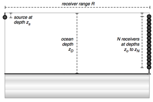
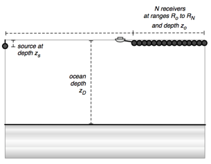
The work focuses on geoacoustic experiment geometries as shown above -- a single source with (possibly multiple) Vertical Line Array(s), and a single source with a Horizontal Line Array of varying length. In both the VLA and HLA cases I study effects of depth and range of the elements upon the quality of the inverted solution. The source sends an acoustic pulse, i.e. the signal is somewhat broadband.
With a few exceptions, the geoacoustic inversion community has largely focused on Bayesian estimation of an ocean bottom described by a handful of parameters – a couple of homogeneous or constant-gradient layers. In the exceptions involving continuous bottom inversion, uncertainty and resolution of the solution are rarely computed and have not been explored deeply, and virtually not at all for the waveform geoacoustic inverse problem. The advantage to considering the problem in terms of waveform inversion is that Parseval’s Theorem shows that a least-squares based objective function can be the same for time domain data, which is considered in this dissertation, as it is for frequency domain data, which has a successful history in the geoacoustic community under the name “matched field inversion”. (Some forms of matched field inversion allow for unknown source spectrum elements – the complete source spectrum is assumed known in this time and frequency domain problem equivalence.) At the same time, waveform inversion in the time domain has a recent history in the seismic inversion literature with success via linearization methods, and full-waveform data provides more information about the model than say travel-time data.
This work effort quantitatively explores the uncertainty, resolution, and regularization in (possibly piece-wise) continuous geoacoustic waveform inversion, to build a framework for quantitatively planning the design of a geoacoustic experiment based on the details of the inversion that the experiment is supporting.
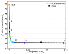
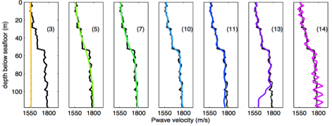
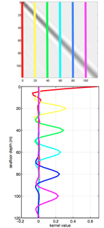
An infinite number of possible P-wave velocity profiles as a function of depth will equally well predict acoustic signals that fit the measured data to within the noise. These solutions have different smoothnesses, all the way from so smooth as to consist of a single straight line (orange profile #3), to having quite a lot of “wiggles” showing far more structure (purple profile #14) than exists in reality (synthetic “reality” being the black jagged line). The best match is somewhere in the middle, and we choose such a middle solution with statistical rigor by using the “L-curve” method of regularization which considers the data/prediction misfit vs. the profile smoothness/roughness on y and x plot axes respectively -- each colored profile is associated with a point on that L-curve.
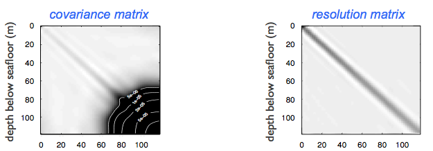
Once the correct solution profile is calculated, the problem is not finished. Uncertainty and resolution of that solution profile are calculated to first order at that solution point via the covariance matrix and resolution matrix of the solution profile. There’s not enough information (never is) in the data to perfectly recover the true bottom profile; what the inversion can recover is a smoothed version of the true profile. The smoothed true profile is related to the original true profile (to first order) by a set of linear functionals, or weighted averages -- the weights are contained in the resolution matrix. The covariance matrix contains the variances and covariances of those weighted averages.
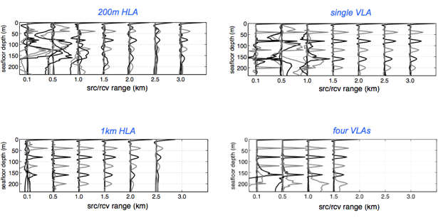
Using these types of results in a “resolution analysis” can be incredibly helpful in planning a new experiment. Below for example are different equipment choices laid out in different geometries, comparing those same resolution kernels, or impulse responses. We see the problem as unstable at close range in both the short HLA and single VLA; simply not enough information is available in the data at those short ranges. (The plot also short at longer ranges the single VLA provides higher resolution velocity results than the short HLA. However, both the long HLA and the four VLAs fix that short-range instability and increase the overall resolution everywhere.
Uncertainty and Resolution in Full-Waveform, Continuous, Geoacoustic Inversion
Andrew A. Ganse, 2013, PhD dissertation, University of Washington geophysics.
(available in PDF, download here, note it’s 21MB)
Abstract: The ocean geoacoustic inverse problem is the estimation of physical properties of the ocean bottom from a set of acoustic receptions in the water column. The problem is considered in the context of equipment and spatial scales relevant to naval sonar. This dissertation explores uncertainty, resolution, and regularization in estimating (possibly piece-wise) continuous profiles of ocean bottom properties from full-waveform acoustic pressure time- series in shallow-water experiments. Solving for a continuous solution in full-waveform seismic and acoustic problems is not in itself new. But analyses of uncertainty, resolution, and regularization were not included in previous works in this category of ocean geoacoustic problem. Besides quantifying the quality of individual inversion results, they also provide an important tool: Methods and details in these topics build to a pre-experiment design analysis based on the problem resolution, which can be estimated without measurements (i.e. before the experiment takes place). The resolution of the bottom inversion is calculated as a function of array configuration, source depth, and range. Array configurations include 40-element horizontal line arrays (HLAs) from 200-1200m long towed at 10m depth, with source range defined as that to closest HLA element, and single and multiple vertical line arrays (VLAs) which cover the water depth. Monte Carlo analyses of the inversion within the local minimum show the extent to which the linear descriptions of uncertainty and resolution used in the experiment design analysis are valid approximations. Since full-waveform geoacoustic inversion is a nonlinear inverse problem, the resolution analysis results are dependent on the choice of bottom model for which they are calculated. Resolution analyses for six widely di↵ering bottom profiles are compared, and at the geometries and frequencies considered in this dissertation, the results and conclusions from the point of view of experiment design decisions are in fact largely similar, with the exception of the presence of a low velocity zone in the bottom model (from which acoustic energy does not return to the receivers). The techniques and conclusions in this work are appropriate when inverting for P-wave velocity profiles in shallow (200m) water, at relatively short (~3km) range with flat bottom, and at low frequency (~100Hz).