
Visualizing GPS tracking data in Python/Jupyter
(Get this Jupyter/ipynb notebook from my Github account)Did you know you can embed interactive Google Maps and other similar mapping tools directly into your Python notebook? Check it out, as we play with and analyze some GPS tracking data! (This Jupyter notebook is availabile for download here.)
To start with, let's go grab some great GPS tracking data to play with. A company called MapMyRun keeps a wonderful database of walking/biking routes in various US cities, based on GPS tracks that users have submitted to the site. From a menu page one can pick from a variety of routes; for example let's pick one walking around the downtown Seattle business district. Note you must create a (free) account on that website to download the track data (the download button at bottom of each page is for climb/altitude data only; the track data comes via the "export this route" link on right of page). After setting up account you can download a GPX file with the track data.
Before getting started we can use a command-line shell utility from the GPXPY package to check the summary stats of the data file:
!gpxinfo route1141462231.gpx
GPX files can contain multiple tracks, each with multiple segments, each with multiple tracking points. For this file the above shows only one track, with a single segment, containing 500 data points. The data files can contain time, altitude, and speed information too, and the above summary suggests those values are missing; we'll double-check that below.
Now for the Python:
# some of this cell's code came from this link - thank you!
# https://ocefpaf.github.io/python4oceanographers/blog/2014/08/18/gpx

import gpxpy
gpx = gpxpy.parse(open('./route1141462231.gpx'))

# Files can have more than one track, which can have more than one segment, which have more than one point...
print('Num tracks: ' + str(len(gpx.tracks)))
track = gpx.tracks[0]
print('Num segments: ' + str(len(track.segments)))
segment = track.segments[0]
print('Num segments: ' + str(len(segment.points)))

# Load the data into a Pandas dataframe (by way of a list)
data = []
segment_length = segment.length_3d()
for point_idx, point in enumerate(segment.points):
    data.append([point.longitude, point.latitude,point.elevation,
                 point.time, segment.get_speed(point_idx)])
import pandas as pd
columns = ['Longitude', 'Latitude', 'Altitude', 'Time', 'Speed']
df = pd.DataFrame(data, columns=columns)
print('\nDataframe head:')
print(df.head())
print('\nNum non-None Longitude records: ' + str(len(df[~pd.isnull(df.Longitude)])))
print('Num non-None Latitude records: ' + str(len(df[~pd.isnull(df.Latitude)])))
print('Num non-None Altitude records: ' + str(len(df[~pd.isnull(df.Altitude)])))
print('Num non-None Time records: ' + str(len(df[~pd.isnull(df.Time)])))
print('Num non-None Speed records: ' + str(len(df[~pd.isnull(df.Speed)])))
print('\nTitle string contained in track.name: ' + track.name)
So we've confirmed the lack of Altitude, Time, and Speed data; just Lon/Lat points. But at least the title string for the track lists total distance and date - the former we can verify with the data; the latter we cannot.
Meanwhile here are some options to get an interactive map plot of the track:
%matplotlib inline
MPLleaflet:
import mplleaflet   # (https://github.com/jwass/mplleaflet)
import matplotlib.pyplot as plt
plt.plot(df['Longitude'], df['Latitude'], color='red', marker='o', markersize=3, linewidth=2, alpha=0.4)
#mplleaflet.display(fig=ax.figure)  # shows map inline in Jupyter but takes up full width
mplleaflet.show(path='mpl.html')  # saves to html file for display below
#mplleaflet.display(fig=fig, tiles='esri_aerial')  # shows aerial/satellite photo
# (I don't actually find the aerial view very helpful as it's oblique and obscures what's on the track.)
Folium:
import folium   # (https://pypi.python.org/pypi/folium)
mymap = folium.Map( location=[ df.Latitude.mean(), df.Longitude.mean() ], zoom_start=14)
#folium.PolyLine(df[['Latitude','Longitude']].values, color="red", weight=2.5, opacity=1).add_to(mymap)
for coord in df[['Latitude','Longitude']].values:
    folium.CircleMarker(location=[coord[0],coord[1]], radius=1,color='red').add_to(mymap)
#mymap   # shows map inline in Jupyter but takes up full width
mymap.save('fol.html')  # saves to html file for display below
Google Maps:
import gmplot   # (https://github.com/vgm64/gmplot)
gmap = gmplot.GoogleMapPlotter(df.Latitude.mean(), df.Longitude.mean(), 14)
gmap.scatter(df['Latitude'], df['Longitude'], 'red', size=7, marker=False)
# apparently cannot be shown inline in Jupyter
gmap.draw("gmap.html")  # saves to html file for display below - hm, see note below about this.
For better display I saved the above to html files which I'll show in subframes below:
%%HTML
<iframe width="45%" height="350" src="fol.html"></iframe>
<iframe width="45%" height="350" src="mpl.html"></iframe>
<!-- <iframe width="45%" height="350" src="gmap.html"></iframe>  hm, this one dies without a Google API key -->
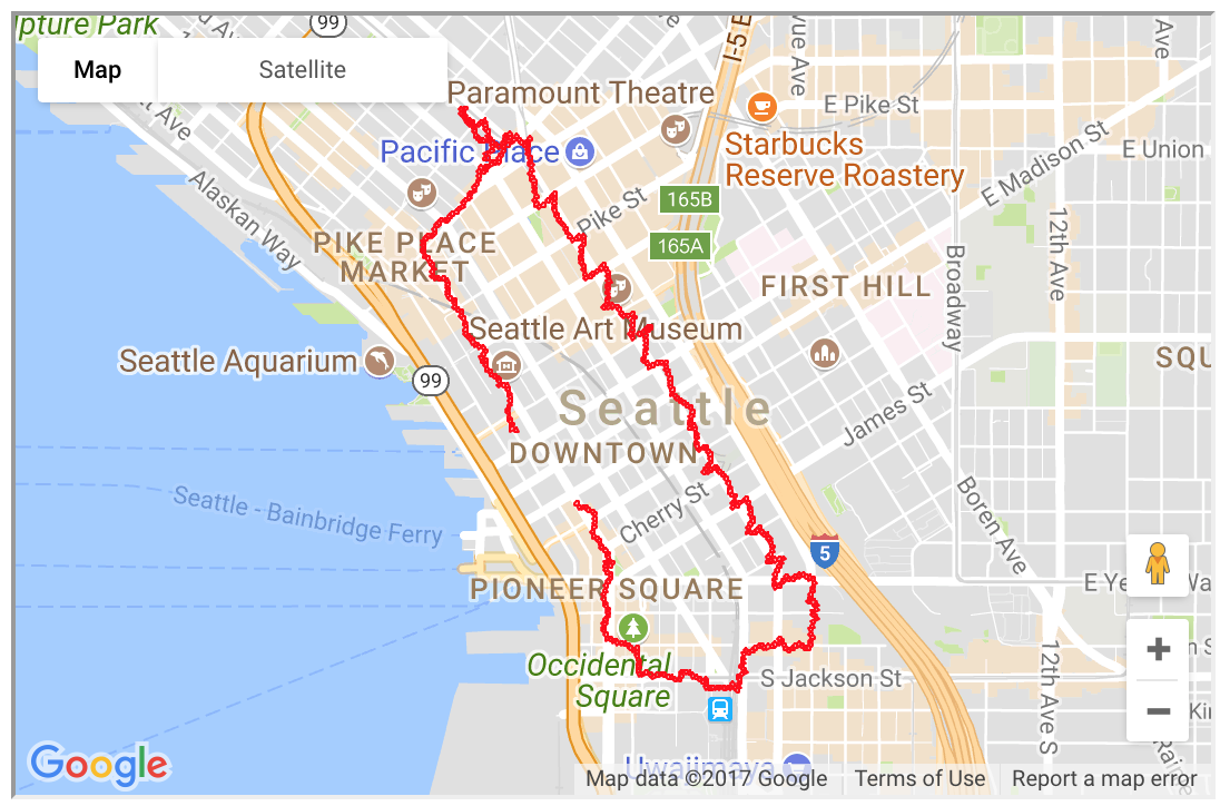
The Google Maps plot below is just the screenshot I took to show how it displayed in my Safari browser outside of Jupyter, actually even using the same <iframe width="45%" height="350" src="gmap.html"></iframe> as above in a separate HTML file (flanked by <HTML><BODY> and </BODY></HTML>), no problem in that case. It appears there's some check they're doing that prevents straightforward anonymous Google Maps calls from within Jupyter, oh well.
%%HTML
<img width="40%" src="gmap.png">
# calculate distances on surface of ellipsoid
from vincenty import vincenty

df['lastLat']=df['Latitude'].shift(1)
df['lastLong']=df['Longitude'].shift(1)
df['dist(meters)'] = df.apply(lambda x: vincenty((x['Latitude'], x['Longitude']), (x['lastLat'], x['lastLong'])), axis = 1) * 1000.

print('Total distance as summed between points in track:')
print('   ' + str(sum(df['dist(meters)'][1:])*0.000621371) + ' mi')
# The df['dist'][1:] above is because the "shift" sets the first lastLon,lastLat as NaN.
print('Comparing to total distance contained in track.name: ' + track.name)
That 0.18 mile difference above is about 274 meters. There may have there been a different instrument or method used by whoever entered that 3.52 into the title string, and also we did not take the elevation changes into account in the distance calculation (the elevation changes were available in that separate download link on the MapMyRun page and I didn't incorporate them into the dataframe here).
However, there's also a very interesting phenomenon going on in the GPS data as seen in those maps above. That walk in downtown Seattle is right among the tallest skyscraper buildings in the city, and the GPS signals are known to reflect off those buildings and cause geometric effects like that for GPS in such downtown areas. There are papers about this - it's not a trivial matter - it's not noise that you can simply filter out, it's a spatially- and temporarily-varying bias, because not only does it depend on where you are standing with your GPS unit downtown, but it also depends on where the GPS satellites are in their trajectory. Here are a few interesting examples from the scientific/engineering literature about this issue: