
From 2008-2015 I participated in the North Pacific Acoustic Laboratory (NPAL), which was a research consortium of multiple universities working together with the Naval Research Laboratory and the Office of Naval Research on problems in long-range ocean acoustics. The focus of our APL group was large-scale statistical data analysis of our measured field data to test the limits of ocean acoustic scattering theories.
Overview
 Acoustic propagation over long ranges (hundreds or thousands of kilometers) in the deep ocean becomes progressively randomized due to ocean variability such as internal waves and "spice" (neutrally buoyant soundspeed fluctuations)
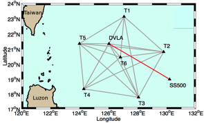
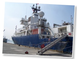 as well as ambient noise, with a direct bearing on Naval capabilities. The consortium conducts major sea experiments to study these topics, the latest being in the Philippine Sea in 2009 and 2010. The Philippine Sea experiment took place about 600km east of Taiwan and Luzon, in five kilometer deep water. The Scripps Institute of Oceanography (SIO) team placed transceivers in a pentagon layout for ocean acoustic tomography investigations, as well as a five-kilometer-long "distributed vertical line array" (DVLA) of hydrophones covering almost the whole water column. Our APL-UW team operated a low-frequency acoustic source system that we lowered from a ship down to a kilometer's depth, transmitting coded signals across 100km (2009) and 500km (2010) to the DVLA so that we could analyze the effects of the internal waves and spice on those acoustic signals along that path.
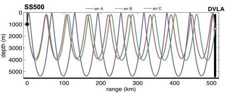 Sound in the ocean does not travel in straight lines, for the speed of sound in the ocean is not constant. Soundspeed in the ocean is governed mainly by the water's temperature and pressure. In the upper kilometer or so the temperature gradually drops with depth so the soundspeed does as well. But at depths below that top kilometer, the temperature remains fairly constant (it's just plain cold!) so the increasing pressure with depth becomes the dominant effect and causes the soundspeed to start increasing with depth again. Thus there is a soundspeed minimum at about one kilometer's depth in the world's oceans, and this has a "waveguide" effect on the sound paths -- the sound waves are guided up and down and up and down again along that 1km deep axis very efficiently for thousands of miles (for low frequencies).
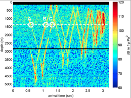
The sound splits up into multiple paths within the waveguide as it travels to the receiver array, at which the pings in the multiple paths come in at different times. It's almost analogous to multiple echoes coming in from walls at different distances, except that here there are no reflections (as with the walls). It is the splitting nature of the waveguide -- differing refraction for differing take-off directions from the source -- that causes the multiple arrivals. The timings of these multiple arrivals are different depending on receiver depth, and when you plot them all together you get a cool accordion-shaped pattern (seen here in real data received on the 5km long vertical array of receivers).
The Navy has taken advantage of these waveguide features of ocean sound propagation since WWII, but the picture is complicated by the fluctuations of internal waves, spice, and ambient noise, which all continue to make it difficult to accurately predict the received fluctuations in ocean acoustic signals. Understanding and better modeling these fluctuations (so they can always be distinguished from targets like submarines) is a longtime interest of the Navy, who funds this work. Yet there are other benefits too -- the oceans are affected by global warming just as are the continents, and sound measurements can be used to study long-term temperature variations in the ocean. Also, "T-phase" energy from oceanic earthquakes gets into that sound axis and can be detected from far away, making these ocean acoustic methods a key tool in studying these earthquakes. In any event, the axis causes sound to split into multiple paths in the ocean, causing the distinctive "accordion" shaped pattern in hydrophone depth vs arrival time plots. This accordion and parts within it shudder and shimmer over time due to the ocean fluctuations, and we use these shudders and shimmers to learn about the ocean fluctuations.
PhilSea2010 acoustic data analysis
One of the major scientific interests in the ocean acoustic research community is to better understand long-range ocean acoustic scattering, in order to explain the phenomenon of deep fading in long-range ocean acoustic propagation. Besides its more esoteric theoretical physics interest in the WPRM -- "wave propagation in random media" -- community, the Navy is also pragmatically interested to understand this fading as a major issue in long-range sonar. Our main focus in the PhilSea experiment was the transmission of low frequency acoustic signals from our ship-dipped sources to SIO's full-ocean-column DVLA receiver array 500km away (see map above).
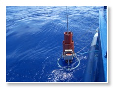 At independent times we lowered our 82Hz source ("HX554") and our dual-band source at 200 & 300Hz ("multiport", shown here), from the ship to one kilometer depth and transmitted for a few days at a time, one ping approximately every 20 seconds. As described above, the sound waves split into the different paths which came into the different arrival branches on the "accordion" (so one whole accordion every 20 seconds).
 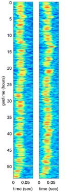 From the accordion we can snip out a single arrival on a single hydrophone (at whatever depth) to analyze the changes in the arrival intensity and position over the 2+ days of the experiment. As it turns out, ocean variability (chiefly from internal waves) causes quite noticeable fluctuations in the signal arrivals over this time period, as seen for example in the plot here which contains two such snipped-out arrivals. While not obvious on this particular plot, when zooming in one sees the signal frequently fade away completely and come back -- i.e. the "deep fading".
There are mathematical theories that predict the statistics of this fading, based on particular assumptions about the ocean variability and about the physical mechanism causing the fading. Our research group has some healthy skepticism about details in these theories, and works to understand when and why and where these theories do work and don't work.
Some other NPAL resources online
The APL-UW NPAL group is one part of the broader NPAL consortium with members from a number of universities and research labs. Some other online material for the NPAL consortium include:
The NPAL website at Scripps Institute of Oceanography (out of date)
The Acoustic Thermometry website at Scripps
Brian Dushaw's (APL-UW) extensive website
APL-UW NPAL website (out of date)
A nicely written up account of ocean acoustic tomography on Wikipedia (I think Brian D. wrote most of this)
Towed CTD Chain
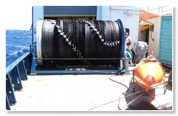
This prototype tool we tried in the PhilSea cruises didn't work very well, but it was an incredibly cool idea with wonderful potential science implications. A completely new version of the tool designed from scratch, developed between SeaBird Electronics and APL-UW, has since performed fabulously and is hoped to provide exciting future science results.
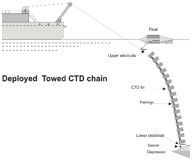
Meanwhile, this tool was a 800m long sea-cable instrumented with 88 individual CTD sensors along its length, each the size of a paperback book. The string of sensors is towed more or less vertically by ship to obtain a 500m deep vertical slice of CTD measurements as far as one tows it. A hydrodynamic depressor at the cable's end holds it down at depth while underway, and a float at surface cutting through waves decouples swell motion tugging on the cable. We added powered control to the big storage drum, developed a special deployment chute and sheave, and worked out quite the deployment and recovery programs.
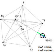
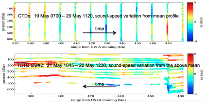
We ran two tows of this cable in the PhilSea in the green and blue colored regions on the map there. Between the two tows we took a week and took over 50 traditional vertical CTD casts across a 500km transect, part of which covered the towpaths. Below are plots of soundspeed fluctuations derived from the CTD information, both from the CTDs (top) and from the very best snippet of the towed CTD chain data we obtained (bottom), after much cleanup and post-recalibration, no salinity data, and estimating the missing pressure data. Blobs of soundspeed structure differ between the two largely due to the time lag between them.
The original interest in these tools is the unprecedented measurement and study of the 2D structure of both internal wave and "spice" variability. "Spice" is neutrally-buoyant soundspeed variation, in which increased salinity cancels the density reduction due to increased temperature, so a blob with greater soundspeed just sits there unlike internal waves. While internal waves have been largely understood for some time now, the generation and propagation and distribution of spice is little known. Towed thermistor chains in the old days only could measure soundspeed and so couldn't separate the effects of spice from the effects of internal waves, as is the current interest with a full-service towed CTD chain.