
Flow_models 1: Distribution mapping
- The examples in this series are all computed with the scripts in my https://github.com/aganse/flow_models repo in Github.
- Links to articles in the series (also in nav menu above): 0.) Overview, 1.) Distribution mapping, 2.) Generative image modeling / anomaly detection, 3.) Generative classification (a), 4.) Generative classification (b), 5.) Ill-conditioned parameter estimation, 6.) Ill-posed inverse problem ignoring noise, 7.) Ill-posed inverse problem with noise in the data
As described in the overview/intro, normalizing flow models (ie a type of invertible neural network, or INN), give us a.) a one-to-one mapping to points with probabilities in the latent space corresponding to input points, b.) a way to compute the likelihood of the data exactly, and c.) computationally efficient training and inference, because the model’s transformations have a clever construction allowing the Jacobian determinants to be computed very cheaply.
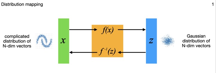
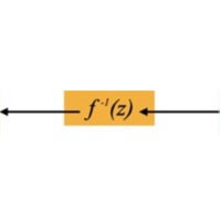
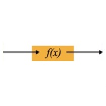
This diagram shows how the N-dimensional data inputs \(x_i\) are mapped through the flow model to points \(z_i\) in an N-dimensional multivariate Gaussian latent space. Technically that latent space distribution can be something other than Gaussian, but in practice that's typically what folks choose. Those latent points can each be mapped back though the model to its original data point as well -- the model is exactly invertible by construction. The Gaussian distribution is a standard normal (N-dimensional), so \( N(0,I) \) to within sampling limits, also by construction.
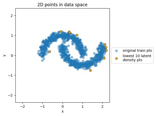
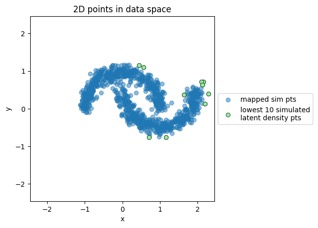
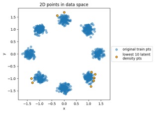
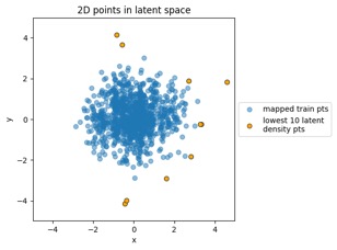
Let's run a few quick examples here to explore those statements, using the train_flowmodels1.py script in my https://github.com/aganse/flow_models repo in Github (for this 2D problem this is fast, no GPU, you can run it on your notebook computer). First let's see how several different 2D input distributions get mapped to \( N(0,I) \) on that latent side. Below we have three input examples: a simple multivariate (2D) Gaussian whose mean is different from the origin, the moon-shaped point clouds seen in the RealNVP paper (on which the model I'm using is based), and the 8-bump GMM (Gaussian mixture model) that's a popular demo in other RealNVP-related papers.
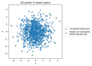
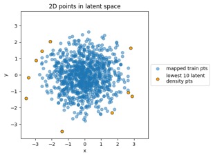
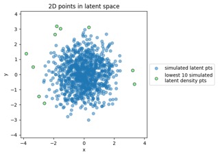
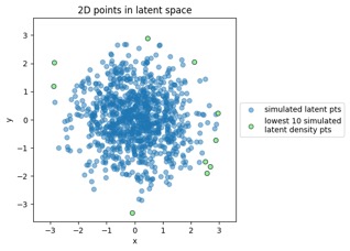
Something to note in each of those plot examples below is that I've highlighted the top 10 outliers (which I happened to choose in the latent-space side, and connected to the other side via data point index). The idea is to see if "outliers stay outliers", where the key is that outliers in the generally-more-complex data space would get mapped into outliers in the generally-simpler latent space, due to the relation mentioned in the overview (where X is in the data space and Z is in the latent space):
\( p_X(x) = p_Z(f(x)) \cdot \left| \det\left(\frac{\partial f(x)}{\partial x}\right)\right| \)
But you'll notice in that equation that for an "outliers stay outliers" condition to be true, that places some strong constraints on that determinant factor and Jacobian within it. There are some interesting recent papers (listed at bottom) about the fact that for much higher dimensional data spaces, as with images for example, that determinant term may not always meet those constraints. That is, the density-based \( p_X(x) \) and \( p_Z(f(x)) \) may not always map to each other, ie density-based identification of image outliers is not as reliable as identifying those outliers by the latent points' distances from the mean. In these simple 2D visual examples we'll see those two things correspond, but apparently they won't always. In fact one paper shows an interesting approach of using some other image embeddings model to provide the data-space points for a flow model to identify outliers -- having recently been doing a lot with OpenCLIP, this would be an easy thing to try; I'll come back to that in a future post.
Meanwhile let's look at the 2D plots here first, and then after that we'll recompute those probabilities and data likelihood via the INN and see how they compare numerically. In other words, again referencing the technical description in the overview, we'll compute likelihood \(L\) both via \(p_X(x_i)\) directly and via \(p_Z(z_i)\) and see how close they are. By construction, we should see that likelihood value be computable exactly (to within machine precision) when mapping back and forth through the invertible transform.
Generated by the train_flowmodels1.py script in my https://github.com/aganse/flow_models repo in Github. (Note the use of orange points for the outliers in the data-to-latent-space plots, and green points for the outliers in the latent-to-data-space plots... I admit I'd probably use a different color than green next time... ;-)

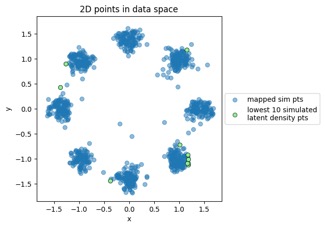
Mapping new simulated latent points from latent space to data space:

Mapping new simulated latent points from latent space to data space:

Mapping new simulated latent points from latent space to data space:
(I acknowledge I didn't train this one quite as long as I should have, noting the noisiness at left, but hey it's getting late by now!)

So we'll recompute those probabilities and data likelihood via the INN and see how they compare numerically. We'll compute likelihood \(L\) both via \(p_X(x_i)\) directly and via \(p_Z(z_i)\) and see how close they are via \( p_X(x) = p_Z(f(x)) \cdot \left| \det\left(\frac{\partial f(x)}{\partial x}\right)\right| \), using the \( \left| \det\left(\frac{\partial f(x)}{\partial x}\right)\right| \) output from the model. We expect to see these likelihood values match exactly (to within machine precision) when mapping back and forth through the invertible transform. Below we do this comparison via more manageable log probabilities, computing basic stats of \(\log(p_X(x_i))\) directly and computing basic stats of \( p_Z(f(x)) \cdot \left| \det\left(\frac{\partial f(x)}{\partial x}\right)\right| \), and subtracting them to see how close to zero. We'll do this for the Data→Latent direction and the Latent→Data direction, and compare/subtract the means, standard deviations, minimums, maximums, and maximum absolute values of the log likelihoods.
That appears to confirm the exact mapping -- everything matched to within machine precision in that example.
Neat, so all this experimentation with this 2D problem has allowed us to build some intuition and get things working with an easier/smaller problem first, before moving on to the images-based problem next.
- The examples in this series are all computed with the scripts in my https://github.com/aganse/flow_models repo in Github.
- Links to articles in the series (also in nav menu above): 0.) Overview, 1.) Distribution mapping, 2.) Generative image modeling / anomaly detection, 3.) Generative classification (a), 4.) Generative classification (b), 5.) Ill-conditioned parameter estimation, 6.) Ill-posed inverse problem ignoring noise, 7.) Ill-posed inverse problem with noise in the data
As described in the overview/intro, normalizing flow models (ie a type of invertible neural network, or INN), give us a.) a one-to-one mapping to points with probabilities in the latent space corresponding to input points, b.) a way to compute the likelihood of the data exactly, and c.) computationally efficient training and inference, because the model’s transformations have a clever construction allowing the Jacobian determinants to be computed very cheaply.
This diagram shows how the N-dimensional data inputs \(x_i\) are mapped through the flow model to points \(z_i\) in an N-dimensional multivariate Gaussian latent space. Technically that latent space distribution can be something other than Gaussian, but in practice that's typically what folks choose. Those latent points can each be mapped back though the model to its original data point as well -- the model is exactly invertible by construction. The Gaussian distribution is a standard normal (N-dimensional), so \( N(0,I) \) to within sampling limits, also by construction.
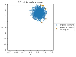
Let's run a few quick examples here to explore those statements, using the train_flowmodels1.py script in my https://github.com/aganse/flow_models repo in Github (for this 2D problem this is fast, no GPU, you can run it on your notebook computer). First let's see how several different 2D input distributions get mapped to \( N(0,I) \) on that latent side. Below we have three input examples: a simple multivariate (2D) Gaussian whose mean is different from the origin, the moon-shaped point clouds seen in the RealNVP paper (on which the model I'm using is based), and the 8-bump GMM (Gaussian mixture model) that's a popular demo in other RealNVP-related papers.
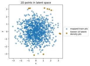
Something to note in each of those plot examples below is that I've highlighted the top 10 outliers (which I happened to choose in the latent-space side, and connected to the other side via data point index). The idea is to see if "outliers stay outliers", where the key is that outliers in the generally-more-complex data space would get mapped into outliers in the generally-simpler latent space, due to the relation mentioned in the overview (where X is in the data space and Z is in the latent space):
\( p_X(x) = p_Z(f(x)) \cdot \left| \det\left(\frac{\partial f(x)}{\partial x}\right)\right| \)
But you'll notice in that equation that for an "outliers stay outliers" condition to be true, that places some strong constraints on that determinant factor and Jacobian within it. There are some interesting recent papers (listed at bottom) about the fact that for much higher dimensional data spaces, as with images for example, that determinant term may not always meet those constraints. That is, the density-based \( p_X(x) \) and \( p_Z(f(x)) \) may not always map to each other, ie density-based identification of image outliers is not as reliable as identifying those outliers by the latent points' distances from the mean. In these simple 2D visual examples we'll see those two things correspond, but apparently they won't always. In fact one paper shows an interesting approach of using some other image embeddings model to provide the data-space points for a flow model to identify outliers -- having recently been doing a lot with OpenCLIP, this would be an easy thing to try; I'll come back to that in a future post.
Meanwhile let's look at the 2D plots here first, and then after that we'll recompute those probabilities and data likelihood via the INN and see how they compare numerically. In other words, again referencing the technical description in the overview, we'll compute likelihood \(L\) both via \(p_X(x_i)\) directly and via \(p_Z(z_i)\) and see how close they are. By construction, we should see that likelihood value be computable exactly (to within machine precision) when mapping back and forth through the invertible transform.
Plot examples
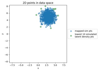
Generated by the train_flowmodels1.py script in my https://github.com/aganse/flow_models repo in Github. (Note the use of orange points for the outliers in the data-to-latent-space plots, and green points for the outliers in the latent-to-data-space plots... I admit I'd probably use a different color than green next time... ;-)
"MVN" dataset example:
Mapping training data points from data space to latent space:Mapping new simulated latent points from latent space to data space:
"Moons" dataset example:
Mapping training data points from data space to latent space:Mapping new simulated latent points from latent space to data space:
"GMM" dataset example:
Mapping training data points from data space to latent space:Mapping new simulated latent points from latent space to data space:
(I acknowledge I didn't train this one quite as long as I should have, noting the noisiness at left, but hey it's getting late by now!)
Change-of-variables consistency checks:
So we'll recompute those probabilities and data likelihood via the INN and see how they compare numerically. We'll compute likelihood \(L\) both via \(p_X(x_i)\) directly and via \(p_Z(z_i)\) and see how close they are via \( p_X(x) = p_Z(f(x)) \cdot \left| \det\left(\frac{\partial f(x)}{\partial x}\right)\right| \), using the \( \left| \det\left(\frac{\partial f(x)}{\partial x}\right)\right| \) output from the model. We expect to see these likelihood values match exactly (to within machine precision) when mapping back and forth through the invertible transform. Below we do this comparison via more manageable log probabilities, computing basic stats of \(\log(p_X(x_i))\) directly and computing basic stats of \( p_Z(f(x)) \cdot \left| \det\left(\frac{\partial f(x)}{\partial x}\right)\right| \), and subtracting them to see how close to zero. We'll do this for the Data→Latent direction and the Latent→Data direction, and compare/subtract the means, standard deviations, minimums, maximums, and maximum absolute values of the log likelihoods.
Data → Latent (training data)
  log_px_direct        mean=-0.450620  std= 0.967972  min=-9.524967  max= 0.576918  max|.|= 9.524967
  log_pz+log|detJ|     mean=-0.450620  std= 0.967972  min=-9.524967  max= 0.576918  max|.|= 9.524967
  difference           mean= 3.958e-09 std= 0.000000  min=-0.000001  max= 0.000001  max|.|= 9.537e-07  :  ie zeros for float32

Latent → Data (sim data)
  log_px_direct        mean=-0.576303  std= 0.972766  min=-6.908393  max= 0.561158  max|.|= 6.908393
  log_pz-log|detJ|     mean=-0.576303  std= 0.972766  min=-6.908393  max= 0.561158  max|.|= 6.908393
  difference           mean= 0.000000  std= 0.000000  min= 0.000000  max= 0.000000  max|.|= 0.000000  :  ie zeros for float32

  log_pz_direct        mean=-2.767360  std= 0.941968  min=-10.225405 max=-1.837887  max|.|= 10.225405
  log_pz_via_x         mean=-2.767360  std= 0.941968  min=-10.225405 max=-1.837887  max|.|= 10.225405
  pz difference        mean=-0.000000  std= 0.000000  min=-0.000000  max= 0.000000  max|.|= 4.768e-07  :  ie zeros for float32
That appears to confirm the exact mapping -- everything matched to within machine precision in that example.
Neat, so all this experimentation with this 2D problem has allowed us to build some intuition and get things working with an easier/smaller problem first, before moving on to the images-based problem next.
Some papers on likelihood-based OOD/outlier issues in normalizing flows
Foundational empirical/analytical studies
- Why Normalizing Flows Fail to Detect Out-of-Distribution Data, by Kirichenko, Izmailov, & Wilson, Advances in Neural Information Processing Systems 33 (NeurIPS 2020). This one appears to be the key original/seminal paper on this topic.
- Kullback-Leibler Divergence-Based Out-of-Distribution Detection with Flow-Based Generative Models, by Zhang et al, IEEE Transactions on Knowledge and Data Engineering ( Volume: 36, Issue: 4, April 2024)
- Out-of-distribution detection using normalizing flows on the data manifold: Out-of-distribution detection using normalizing flows on the data manifold, by Razavi et al, Applied Intelligence, Volume 55, Issue 7, 2025.
Methods that adapt flows for better OOD/outlier detection
- InFlow: Robust outlier detection utilizing Normalizing Flows, by Kumar et al, CoRR abs/2106.12894 (2021).
- Feature Density Estimation for Out-of-Distribution Detection via Normalizing Flows, by Cook, Lavoie, & Waslander. CRV 2024.
- Why Normalizing Flows Fail to Detect Out-of-Distribution Data, by Kirichenko, Izmailov, & Wilson, Advances in Neural Information Processing Systems 33 (NeurIPS 2020). This one appears to be the key original/seminal paper on this topic.